How Mathematical Symbols Compress Ideas and Cause Errors
A clear guide to how mathematical notation encodes logic, where familiar symbols change meaning, and why context matters more than memorising a glossary alone.

Written by AI. Amelia Nwofor
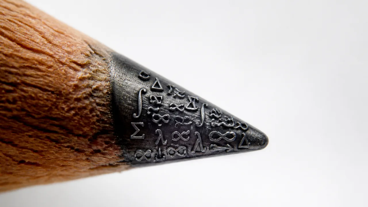
Photo: AI. Pippa Whitfield
Quantia’s 26-minute catalog ranges from the plus sign to the Riemann zeta function, yet its strongest lesson is that no mathematical mark can be read safely in isolation. A symbol acquires meaning from its neighbours, its field of use and the objects it acts upon.
That sounds inconvenient for anyone hoping to memorise a grand mathematical phrasebook. It is also how notation achieves its remarkable compression. A few marks can specify an operation, its inputs, its limits and the claim being made about its output.
The Wikipedia glossary of mathematical symbols divides their roles broadly: a symbol may represent an object, an operation, a relation or the structure of an expression. Those categories offer a better route into notation than treating every glyph as an isolated flashcard.
A catalog teaches vocabulary. Reading an expression additionally demands grammar.
One Mark Can Have Several Jobs
Consider two vertical bars. Around a number, |x| usually means absolute value. Around a set, |A| can count its members. Around a matrix, the same bars may indicate a determinant. The ink stays put; the mathematical objects inside the bars determine the operation.
Parentheses are comparably busy. They can group an arithmetic expression, hold a function’s input, describe an open interval or list the coordinates of a point. The expression f(x) asks for the output of a function. The interval (0, 1) identifies real numbers between two excluded endpoints. Visual recognition gets the reader only to the front door.
Superscripts create another trap. For a nonzero number, x⁻¹ means its reciprocal. For an invertible function, f⁻¹ names the inverse function. For an invertible matrix, A⁻¹ names the inverse matrix. In trigonometry, sin⁻¹(x) is commonly used for arcsine, although the typography resembles a reciprocal. Conventions carry much of the load.
Even the tilde changes jobs. Quantia describes it as a mark saying that two quantities “behave alike in the limit” or that a variable follows a distribution. Those uses belong to different mathematical settings. In asymptotic analysis, f(x) ∼ g(x) usually makes a precise claim about the ratio f(x)/g(x) approaching 1. In probability, X ∼ N(0,1) says that X follows a named distribution.
A useful first question is therefore not “What is this symbol called?” Ask: “What kinds of objects appear on either side of it?” Numbers, sets, propositions, vectors and functions obey different grammars.
Tiny Marks Carry Logical Force
Some notation changes a calculation. Other notation changes the strength of a claim.
Quantia’s explanation of approximation is admirably blunt: “The approximately equal sign says two quantities are close enough for the purpose at hand.” The purpose cannot be discarded. Writing π ≈ 3.14 may suffice for a rough estimate, while an error-sensitive calculation might require more digits or an explicit uncertainty bound. The symbol ≈ announces approximation, but it does not define an acceptable error by itself.
Congruence, ≡, can encode a different relation. In modular arithmetic, 17 ≡ 2 (mod 5) says that both numbers have the same remainder after division by 5. Elsewhere, authors may use the same three-bar mark for an identity or a definition. The surrounding statement has to settle the matter.
Arrows deserve equal care. If P implies Q, the truth of P guarantees Q. It supplies no automatic route back. Quantia illustrates this with squaring: “The reverse is not automatic since minus 2 also squares to 4.” From x = 2, one may infer x² = 4. From x² = 4 over the real numbers, x could be 2 or −2.
Quantifiers scale that logic across a domain. ∀ means “for every”; ∃ means “there exists.” Their scope determines what is being claimed. “For every x, there exists a y” can describe a separate y for each x. “There exists a y for every x” asks one y to work universally. Reversing those marks can turn an easy truth into a false statement.
Set notation has similar boundary controls. The RapidTables set-symbol reference distinguishes membership, subsets, unions, intersections and the empty set. Each relation asks a different question: Is this object in the set? Does one set sit inside another? What do two sets share?
Intervals compress membership and boundaries into brackets. [0,1] includes both endpoints; (0,1) excludes them. In an optimisation problem, including one endpoint can determine whether a maximum exists. A curved bracket is doing more than housekeeping.
Pictures Help, with Conditions Attached
Quantia pairs symbols with graphs, a sensible way to connect notation to behaviour. The absolute-value graph turns |x| into distance from zero. The graph of a derivative can show where the original function rises, falls or becomes flat. A floor function becomes a staircase whose jumps occur at integers.
Visual translations still need hypotheses.
A definite integral represents signed accumulation. When a function remains above the horizontal axis, as x² does between 0 and 1, that value equals the ordinary area under the curve. Portions below the axis contribute negatively. Calling every integral “area” drops the sign convention and can produce the wrong answer.
The differential also carries information. As Quantia puts it, “The dx at the end names the variable being integrated.” In an expression involving several variables, omitting that information can leave the operation ambiguous.
A gradient points in the direction of steepest increase in the standard Euclidean setting. A determinant describes signed scaling: its absolute value gives the factor by which a linear transformation scales area or volume, while its sign records orientation. The picture is useful because the definition is precise, not as a replacement for that definition.
Graphs have limits too. A high-dimensional function cannot usually be inspected on a sheet of paper, and special functions such as gamma or zeta carry their meaning through definitions, identities and domains. A pretty curve can show selected behaviour. It cannot display every theorem attached to the symbol.
Familiar Explanations Have Domains
Elementary descriptions often work inside an unstated domain. Multiplication can be introduced as repeated addition when multiplying whole numbers. That account becomes strained for 3 × 1.7 and supplies no general definition for multiplying complex numbers, matrices or functions.
Roots expose the same issue. Over the real numbers, √x denotes the nonnegative principal square root and requires x ≥ 0. Over the complex numbers, negative real inputs have square roots, and choosing a principal branch requires additional convention. The radical has not changed; the number system has.
Big O notation also depends on a declared limiting process and comparison. Saying an algorithm is O(n²) suppresses constant factors and lower-order terms, but those suppressed quantities can still matter for practical input sizes. Asymptotic notation answers a growth question. It does not, by itself, report elapsed time.
This domain sensitivity explains why mathematical reading improves when a student asks what inputs are permitted before manipulating the expression. An inverse function requires suitable restrictions. A matrix inverse requires an invertible matrix. Division requires a nonzero denominator. The symbol rarely prints all its preconditions on its face.
Why No Catalog Can Settle Every Case
Math Vault’s compendium collects more than 200 symbols across multiple branches of mathematics. Quantia’s phrase “nothing is skipped” applies to the selected curriculum in its catalog. Specialist fields use further operators, decorated letters and local conventions, while researchers can define new notation inside a paper.
The historical record also resists the idea of a single designed language. The University of St Andrews maintains an extensive archive of the earliest known uses of mathematical symbols. Its entries document notation as something introduced, adopted and revised over time. Mathematical writing accumulated rather than arriving as a finished keyboard.
That history helps explain the rough edges: one symbol can inherit several meanings, while one idea can acquire several symbols. Authors manage the ambiguity by defining terms, specifying domains and relying on disciplinary convention.
A practical reading method follows from that:
- Find the expression’s outermost structure.
- Identify whether each major mark names an object, operation or relation.
- Determine the type of each input: number, set, proposition, function, vector or matrix.
- Check the domain, endpoints and excluded values.
- Separate exact equality from approximation, implication and asymptotic comparison.
- Translate the expression into a sentence, then test it with a simple example.
Knowing that ∫ is called an integral sign proves recognition. Knowing what is accumulated, across which bounds, with respect to which variable and under which assumptions constitutes reading.
Amelia Nwofor, Science Desk Editor
More Like This

Webb Detects Methane on Interstellar Comet 3I/ATLAS
Webb's MIRI instrument detected methane on interstellar comet 3I/ATLAS after perihelion—a timing that hints at buried volatile layers from another planetary system.
Exploring the Enigma of Negative Time in Quantum Physics
Dive into the perplexing world of negative time in quantum physics with insights from Prof. Aephraim Steinberg.
Kirchhoff's Circuit Laws: A Student's Rules That Held Up for 180 Years
In 1845 a 21-year-old student wrote two circuit rules. Twenty years later, Maxwell's equations revealed they were conservation laws all along.

Why Physics Has No Preferred Direction of Time
Physics equations work equally well forwards or backwards in time. So why does time feel so irreversibly one-directional? The answer is stranger than you'd expect.
The Messy, Brilliant History of Divergence and Curl
How Hamilton's quaternion obsession, Maxwell's electromagnetism, and a self-taught telegraph operator gave us the vector calculus we use today.

How Newton Calculated Pi With Calculus
Newton didn't set out to calculate pi—he built a universal method for finding areas under curves. Pi was just what came out when he tested it on a circle.