How TimescaleDB Keeps Time-Series Summaries Current

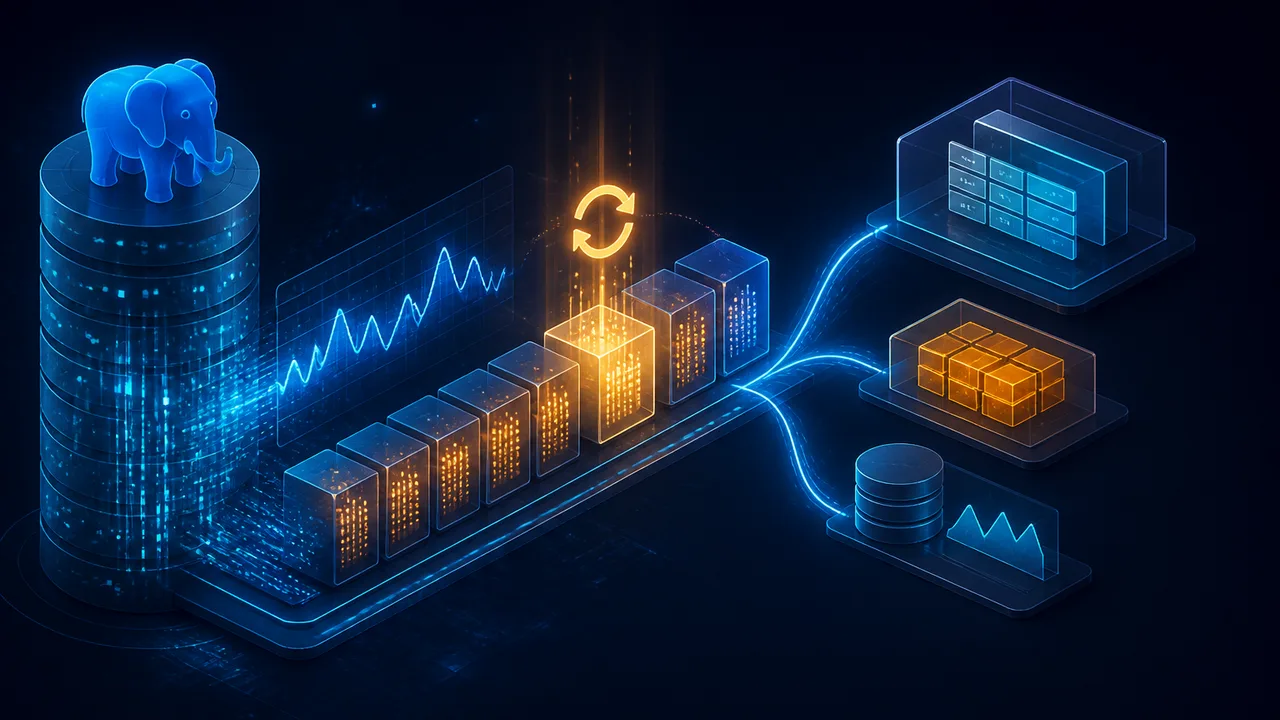
TimescaleDB 2.28.0 processes continuous-aggregate refresh windows in batches of 10 time buckets by default. That detail sounds like release-note furniture, but it exposes the feature’s governing idea: the database can maintain a time-series summary without rebuilding its entire history whenever recent data changes.

For dashboards built around hourly request counts, daily sensor averages or other stable time buckets, this offers a middle route between PostgreSQL’s full materialized-view refresh and a separate analytical database. The trade is precision for bounded work. TimescaleDB can recompute an affected bucket, while a general incremental-view-maintenance system may propagate a smaller delta and an analytical engine may scan the underlying data faster.

Choosing among them requires asking where the system should pay: during writes, refreshes or reads, or in the operational plumbing between databases.

PostgreSQL’s Full-Replacement Baseline

PostgreSQL’s version 9.3 documentation described REFRESH MATERIALIZED VIEW with admirably blunt language: it “completely replaces the contents” of the view. The backing query runs again, the old contents go away and the refreshed result becomes available.

That historical baseline explains why materialized views can become awkward as source tables grow. A cached summary makes reads cheaper, but refreshing it can revisit data whose contribution has not changed. The database has moved computation away from dashboard users and into a scheduled maintenance job. It has not made the computation disappear. Databases remain stubbornly opposed to free lunch.

Incremental view maintenance, usually shortened to IVM, attacks that repeated work. A technical overview of IVM describes the general approach as processing the affected delta rather than reprocessing the full dataset. It also traces modern implementations through timely dataflow, differential dataflow and DBSP, approaches intended to support more expressive computations than a narrow summary-table mechanism.

TimescaleDB continuous aggregates occupy a more opinionated point on that spectrum. Time already divides the data into buckets, so the extension has an obvious unit of repair: recalculate the bucket touched by a change. That unit can include many rows, making it coarser than general delta propagation. It is also easier to reason about for workloads whose questions already sound like “requests per hour” or “maximum temperature per day.”

The Bucket is the Contract

Tiger Data’s refresh documentation says a continuous aggregate materializes values such as minimums, maximums and averages into time buckets. Only buckets that fit completely inside a requested refresh window are refreshed; incomplete buckets are excluded.

The function can use tracked changes to bound work. If the window boundaries are null after the initial refresh, the lowest and highest changed elements define the range. Since version 2.28.0, the manual refresh function divides that range into batches by default. Each batch runs in its own transaction, releasing locks and exposing results between batches. Setting buckets_per_batch to zero restores a single atomic pass across the window.

Those choices create a consistency decision for the operator. Smaller transactions reduce how long locks are held and let fresh batches appear sooner, but readers may observe a refresh in progress rather than one all-at-once replacement. A single pass gives readers an atomic window while asking the database to carry a larger transaction. Dashboard operators therefore have to choose between gradual visibility and a synchronized cutover.

Refresh windows also encode an application assumption about lateness. If events or corrections can arrive well after their timestamps, the policy must reach far enough back to revisit their buckets. Tiger Data’s refresh reference explains changed-element tracking and window boundaries, but it does not supply a universal late-arrival policy for every workload. Teams should test their own correction patterns instead of treating “continuous” as a promise that every historical value updates immediately.

A 2022 Mindee engineering example illustrates the policy model with an hourly API summary refreshed every 10 minutes across the previous two hours. That configuration is an example rather than a current default, and its two-hour horizon would be an application choice. It works when expected corrections fall inside that horizon. Older changes require a wider policy or an explicit refresh.

One documented edge case deserves a Post-it on the monitor. Tiger Data warns that a refresh may skip buckets when changes occurred only in a secondary table used by a JOIN. The time-series source can remain untouched while dimension data changes underneath the aggregate. If customer names, device metadata or pricing classifications participate in the result, developers need an explicit strategy for refreshing those effects. “The source row changed” becomes a multi-table question, and the invalidation machinery does not infer every answer.

General IVM Buys a Different Kind of Flexibility

A general IVM engine aims to transform changes through a query rather than treating time buckets as the primary repair boundary. That can suit continuously updated joins, nested computations or results whose natural grouping has little to do with time. The same flexibility introduces harder implementation problems. The IVM overview notes that conventional relational delta techniques become more expensive for complex or computationally demanding queries, especially recursive or nested structures.

Continuous aggregates therefore make a narrower bargain. When the query naturally groups by time and tolerates bucket-level recomputation, the database can avoid the machinery of a broader dataflow system. When updates must propagate through arbitrary relationships with tighter freshness requirements, teams should benchmark a purpose-built IVM engine against the queries they actually run.

The available comparisons do not include a controlled benchmark running the same query through TimescaleDB and a general IVM engine. Bucket-level work should not be assumed faster merely because its model is narrower. Query shape, changed-data distribution, indexes and hardware can reverse an architectural rule of thumb with impressive efficiency.

Leaving Postgres Moves the Bill

A separate analytical engine offers another answer: copy the data into storage designed for scans and aggregations. The gain can be large, but somebody must operate synchronization, validation, retries and recovery after the benchmark chart has left the meeting.

A MariaDB.org experiment using DuckDB-backed analytical snapshots loaded 3 million generated order and order-item rows in 34.492 seconds. Its complete report fell from 18.464 seconds with InnoDB tables to 0.292 seconds when both analytical tables used DuckDB. The author explicitly limited the result to one machine, one Docker environment and one report shape, with cache state not formally controlled.

The snapshot did not update itself. A production version would need refreshes, incremental synchronization, change-data capture or ETL, plus validation and failure recovery. Continuous aggregates avoid that second-system workload by keeping raw data and summaries in the PostgreSQL environment, although they cannot provide every capability of a separate analytical engine.

Purpose-built engines can also have a substantial advantage when the workload needs raw-row export rather than compact summaries. In a QuestDB-run egress benchmark, TimescaleDB’s ADBC path reached 14 million rows per second, compared with 94 million for ClickHouse’s fastest streaming path and 220 million for QuestDB. The vendor disclosed that the TimescaleDB dataset contained 458 million rows rather than the intended 500 million and said rates were calculated from rows actually received.

That benchmark measured a full-table, five-column transfer with no filtering, joins or aggregation. It cannot rank continuous-aggregate performance. It instead marks the boundary of the feature’s value: precomputed buckets help when the application wants a small summary; they do not turn PostgreSQL’s row-oriented storage and wire path into a purpose-built bulk analytical engine.

A Decision Based on the Shape of the Question

Continuous aggregates fit best when four conditions line up:

1. The source already lives in TimescaleDB or PostgreSQL, and another data system would add unwanted synchronization work.
2. The dominant queries reduce data into stable time buckets.
3. Refresh latency can be expressed as a policy, including a deliberate window for corrections.
4. Joined secondary-table changes and incomplete buckets can be handled explicitly.

General IVM becomes more attractive when arbitrary relational changes must flow into results continuously. A separate analytical database can justify its extra pipeline when users need broad scans, high-cardinality exploration or bulk extraction that pre-aggregation cannot answer.

The cheapest architecture is rarely the one with the fastest isolated query. It is the one whose maintenance boundary matches the data’s pattern of change. TimescaleDB draws that boundary around time buckets, and teams should choose it only when their application draws roughly the same line.